| 일 | 월 | 화 | 수 | 목 | 금 | 토 |
|---|---|---|---|---|---|---|
| 1 | 2 | 3 | 4 | 5 | ||
| 6 | 7 | 8 | 9 | 10 | 11 | 12 |
| 13 | 14 | 15 | 16 | 17 | 18 | 19 |
| 20 | 21 | 22 | 23 | 24 | 25 | 26 |
| 27 | 28 | 29 | 30 |
- 시뮬레이션
- 포탑부수기
- 구현
- PQ
- 3Dreconstruction
- DP
- 조합
- 수영대회결승전
- 슈퍼컴퓨터클러스터
- 나무박멸
- dfs
- ARM
- 마이크로프로세서
- 코드트리빵
- 마법의숲탐색
- 토끼와 경주
- Calibration
- 순서대로방문하기
- ros
- 삼성기출
- ICER
- 소프티어
- 이진탐색
- BFS
- DenseDepth
- 싸움땅
- 백준
- 왕실의기사대결
- 루돌프의반란
- 코드트리
- Today
- Total
from palette import colorful_colors
[Computer Vision] SGBM을 이용한 Disparity Map 구하기와 meshlab을 이용한 3D reconstruction 본문
[Computer Vision] SGBM을 이용한 Disparity Map 구하기와 meshlab을 이용한 3D reconstruction
colorful-palette 2023. 6. 22. 16:47이번 포스팅에선 Opencv의 StereoSGBM을 이용해 disparity map을 구하고, meshlab 프로그램을 이용해서 3D reconstruction을 구하는 과정을 담았습니다.

(사용한 left, right 이미지)
<이미지 정보.txt>
cam0=[998.834 0 327.302; 0 998.834 245.534; 0 0 1]
cam1=[998.834 0 368.275; 0 998.834 245.534; 0 0 1]
doffs=40.973
baseline=203.047
width=701
height=487
ndisp=143
1. Disparity map 구하기:
Code:
import os
import cv2
import numpy as np

#left_image_path = './Newkuba/im0.png'	# left 이미지 가져오기
#right_image_path = './Newkuba/im1.png'	# right 이미지 가져오기

# 이미지 gray scale로 읽기
left_image = cv2.imread(left_image_path, 0)
right_image = cv2.imread(right_image_path, 0)

# StereoSGBM Parameter 설정
stereo = cv2.StereoSGBM_create(blockSize = 7, numDisparities = 96, speckleWindowSize= 100, speckleRange = 100)

# disparity map 계산
disparity = stereo.compute(left_image, right_image)

# 0~ 255로 Normalize하기
disparity_normalized = cv2.normalize(disparity, None, alpha=0, beta=255, norm_type=cv2.NORM_MINMAX, dtype=cv2.CV_8U)


cv2.imshow("Disparity image", disparity_normalized)
cv2.waitKey(0)
cv2.destroyAllWindows()
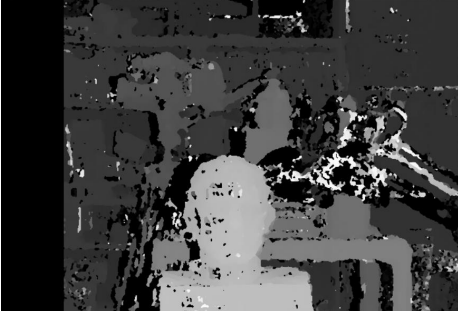
파라미터를 수정하여 disparity map을 조절했고( blockSize = 7, numDisparities = 96, speckleWindowSize= 100, speckleRange = 100) 이후 0~255까지 normallize를 이용해서 png파일을 생성했습니다. 색깔이 밝으면 가깝고, 어두우면 먼 거리를 나타냅니다.
완성된 Disparity map:
2. 3D reconstruction 하기
code:
import cv2
import numpy as np
# Data
focal_length = 998.834
baseline = 203.047
ox = 327.302
oy = 245.534
left_image_path = './Playroom/im0.png' # 왼쪽 이미지 가져오기
right_image_path = './Playroom/im1.png' # 오른쪽 이미지 가져오기
color_image = cv2.imread('./Playroom/im0.png') # 색상을 위한 이미지. 단순히 왼쪽 이미지를 가져옴.
left_image = cv2.imread(left_image_path, 0)
right_image = cv2.imread(right_image_path, 0)
# StereoSGBM Parameter 설정
stereo = cv2.StereoSGBM_create(blockSize = 7, numDisparities = 96, speckleWindowSize=
100, speckleRange = 100)
# disparity map 계산
disparity = stereo.compute(left_image, right_image)
# 0~ 255 로 Normalize 하기
disparity_normalized = cv2.normalize(disparity, None, alpha=0, beta=255,
norm_type=cv2.NORM_MINMAX, dtype=cv2.CV_8U)
# disparity 를 이용해서 Z 구하기
D = disparity
D = np.where(D == 0, 1, D) # 0 으로 나눠지는 것을 막기 위해 0 을 1 로 바꿈
Z = focal_length * baseline / D
Z = cv2.normalize(disparity, None, alpha=0, beta=255, norm_type=cv2.NORM_MINMAX,
dtype=cv2.CV_8U)
# X, Y, Z, R, G, B 를 저장하기
points = []
for i in range(disparity.shape[0]):
for j in range(disparity.shape[1]):
X = j
Y = i
r = color_image[i, j, 0]
g = color_image[i, j, 1]
b = color_image[i, j, 2]
points.append(f"{X} {Y} {Z[i,j]} {r} {g} {b}")
# disparity 값을 txt 파일에 저장
with open('output.txt', 'w') as f:
for point in points:
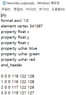
f.write(f"{point}\n")코드를 실행하면 "X Y Z r g b" 정보가 픽셀 수만큼 있는 output.txt 파일이 생성됩니다.
이제다음과 같이 header를 추가해주고, 확장자를 ply로 바꿔 저장해줍니다. (element vertex 수는 픽셀 수 - 가로 x 세로)
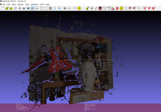
이제 meshlab을 이용해서 3d reconstruction을 해봅시다.
다음 링크에서 meshlab 프로그램 다운 가능:
MeshLab
--> MeshLab the open source system for processing and editing 3D triangular meshes. It provides a set of tools for editing, cleaning, healing, inspecting, rendering, texturing and converting meshes. It offers features for processing raw data produced by 3D
www.meshlab.net
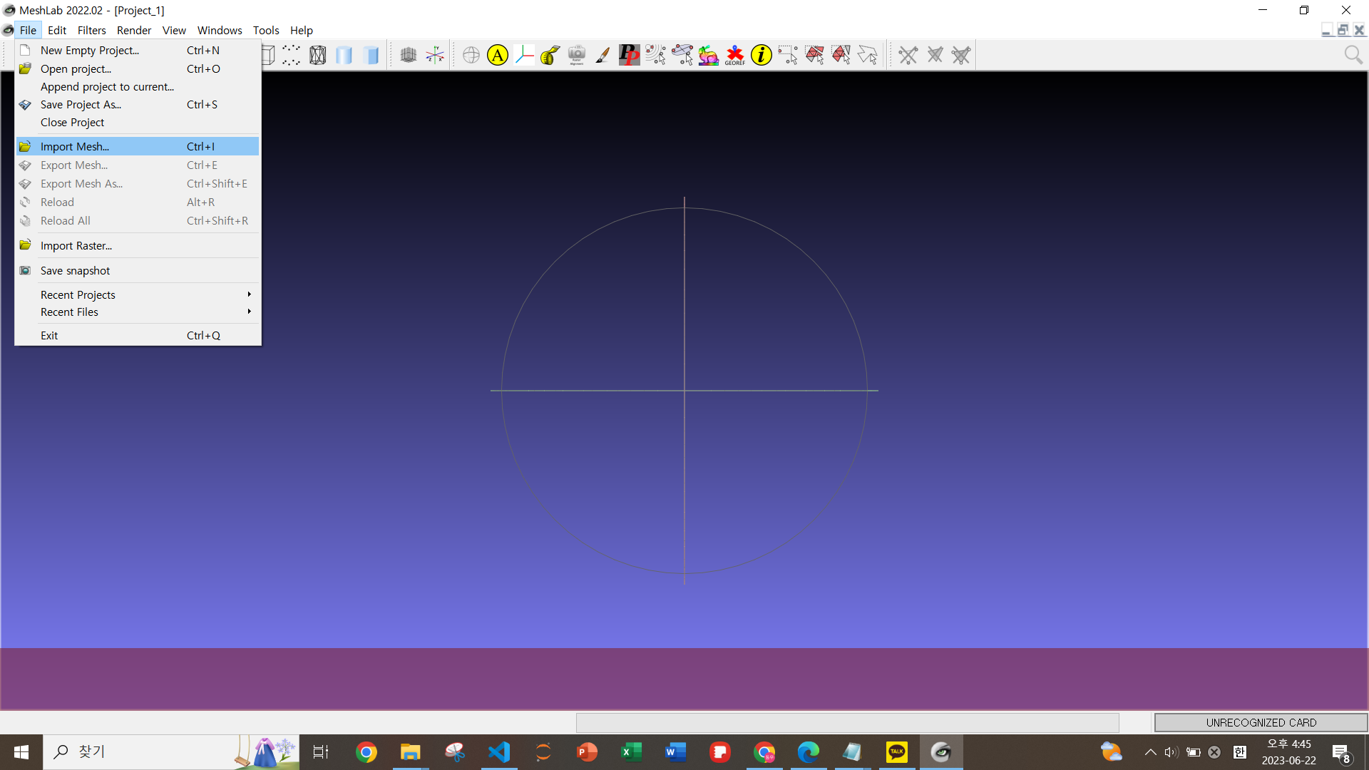
meshlab을 들어가면, 다음과 같은 빈 화면에서 File - import mesh로 들어가 준비된 ply를 선택해서 넣어주면 3d reconstruction된 모습을 볼 수 있습니다.
최종 결과물:
'AI > Computer Vision' 카테고리의 다른 글
| [Computer Vision] Homography를 이용한 파노라마 만들기(python 코드 첨부) (0) | 2023.05.17 |
|---|---|
| [Computer Vision] opencv를 이용해 templete matching 구현하기 (0) | 2023.05.06 |
| [Computer Vision] Calibration이란?, Intrinsic parameter, extrinsic parameter (0) | 2023.04.18 |
| [Computer Vision] Aperture(조리개), DoF(심도) (0) | 2023.03.20 |
| [Computer Vision] SLR, Pinhole(핀홀 카메라), Focal length(초점거리), 렌즈공식 (0) | 2023.03.20 |


